Microsoft Excel offers many advanced shortcuts, formulas, and functions to learn and apply.
Whether you are an Excel beginner or possess moderate Excel tips, here are Excel hacks to evolve your knowledge and amp up your Excel game.
What is Excel?
Microsoft Excel is a data analysis, visualization, and data validation spreadsheet software that helps business professionals store data and track critical business datasets with simple to advanced formulas.
Excel uses spreadsheets to optimize businesses’ data operations without affecting your data integrity.
Regardless of the type of industry, all departments, including sales, marketing, finance, operations, technology, and human resources use Excel.
While the use cases differ for each business department, knowing practical Excel hacks and tricks to generate your chosen report, dashboard, and statements will help.
25 Excel Hacks for Every Use Case
If you are reading this, you must be aware of the Excel basics, like:
- Adding, subtracting, multiplying, and dividing numbers
- Adding or deleting multiple rows, all the columns, one cell, and multiple cells
- Adding colors, highlighting numbers, blank cells, rows, and columns
Since most people know how to carry out these functions, we won’t bore you with that. Let’s discuss the advanced Excel hacks to take your skills to the next level.
We have segregated the Excel hacks and tricks into three categories:
- Keyboard shortcuts, formulas, and functions: For all the functions and formulas to conduct extensive and calculated calculations within minutes
- Productivity boosters: To help you convert your Excel sheets into a productivity machine
- Optimizing spreadsheets: Help you optimize your spreadsheet with minimum work and get better at data validation
Keyboard shortcuts, formulas, and functions
Below are the keyboard shortcuts every Excel enthusiast must know:
1. Entering the number as a text
In situations where you want to feature numbers in a readable format, use this shortcut—add an apostrophe (‘) before the number.
2. Selecting a portion of data at once
When dealing with a huge dataset, if you want to select a particular portion of the data:
- Add the first cell or fill up one cell
- Press the ‘Ctrl Shift’ buttons together and scroll down
- Click the last cell
3. Open more than one file at once
Want to open multiple Excel files in one go? Here’s how to do so:
- Click the ‘File’ tab and then ‘Open’ in the top data tab
- Hold the ‘Ctrl’ button and select all the files
- Now click on ‘Open’
4. Autofill technique
Tired of right-clicking every time and clicking on ‘Paste Special’ to add missing information?
Excel sheet fills in missing information in a data series. Suppose you make a series of even numbers and fill in the first three numbers in an entire column.
- Select the first three numbers
- Drag your cursor down to the bottom right corner until a ‘+’ sign appears
- Now drag the cursor down based on the serial numbers you are looking for

5. Simplify data visibility with the ‘Transpose’ feature
Suppose a long column filled with large datasets confuses you. A great way to simplify your view is to convert these columns into rows (and vice versa). This will help you organize your entire worksheet and establish straightforward visibility.
Why go for the same old route of using ‘Paste Special’ to create the rows manually when the Transpose feature does the job?
- Select the rows/columns/multiple cells you want to transpose
- Right-click to ‘Copy’ these datasets
- Select the columns/rows where you want to see the new data view
- Now right-click again and click on ‘Paste Special’
- In the ‘Paste Special’ window, scroll down to check the ‘Transpose’ box
6. Create simple charts and graphs
Creating simple marketing and sales dashboards is easy with Microsoft Excel. An Excel sheet allows you to create simple bar charts, line graphs, and pie charts for selected datasets. Add a table within Excel or copy the datasets and ‘Paste Special’ to create charts.
- Select the datasets in multiple cells
- Click ‘Insert’ followed by ‘Recommended Charts’
- In the ‘Recommended Charts’ window, you will find all the chart types Excel recommends for the highlighted datasets
- Pick the most convenient chart type and click on ‘OK’
- Use ‘Chart Elements,’ ‘Chart Styles,’ and ‘Chart Filters’ to customize your charts by changing axes and adding colors and data labels
The ‘Save as a Template’ feature lets you save chart templates for future use instead of creating them from scratch each time.

7. Add filters
If users want to view a particular row or column, Excel allows them to filter out the remaining data from the spreadsheet.
To do this:
- Click on the ‘Sort and Navigation’ bar in the top data tab
- In the Drop-down window, select how you want to filter the datasets, like A to Z or Z to A, or customized sorting

8. Select unlinked cells and format cells
Want to select multiple cells from different columns or rows instead of double-clicking ‘Paste Special’ over and over?
Click on the ‘Ctrl’ key and select the specific cells.
Another great Excel hack is to format cells by:
- Right-click in the Home tab
- Click on ‘Cell Styles’
- Click on ‘Modify’ followed by ‘Format’ to format cells and change the content as you want
The ‘Format Cells’ feature improves the clarity and readability of data presentation.
9. Create a personalized shortcut menu
If you are a dedicated Excel user and open Excel files daily, customize your Excel ribbon so you don’t have to look for shortcuts every time.
- Go to ‘File’ and select ‘Options’
- Now click on the ‘Quick Access Toolbar’
- Add all the functions that are a must for your daily Excel operations
- Click ‘Save’
📚Pro tip: Consider using pivot tables to summarize entire data quickly.
To create pivot tables, select any one of the blank cells, click on ‘Insert,’ and then Click on ‘Pivot Table.’
A pivot table and a personalized shortcut menu will help you get a detailed understanding of a complicated dataset. Adding a pivot table to Excel reports is common for sales and marketing professionals.
10. Five major Excel functions and their applications
Here is a quick glimpse into the five most useful Excel functions and how to use them:
- IF: This function performs a logical test to help the user return to one value if the condition is true or to the other if the condition is false
Syntax – IF(logical_test, value_if_true, [value_if_false])
- INDEX: The function returns to a particular value or one of the first cell references from a data array
Syntax – INDEX(array, row_num, [column_num])
- VLOOKUP function/HLOOKUP function: The VLOOKUP function lets you search for data in the rows of your spreadsheet, and HLOOKUP allows you to search for data in the columns
VLOOKUP Function Syntax -VLOOKUP(lookup value, table array, column number, Approximate match (TRUE) or Exact match (FALSE))
HLOOKUP Syntax – VLOOKUP(lookup value, table array, row number, Approximate match (TRUE) or Exact match (FALSE))
- MATCH: This Excel function searches for a particular item in multiple cells and returns the item in a relative position within the same range
Syntax – MATCH(lookup value, lookup array, [match type])
- COUNTIF: This function counts the number of cells that meet criteria or have the same value
Syntax – COUNTIF(range, criteria).
11. Eliminate duplicate datasets
Long-range datasets tend to have duplication. For example, if you are trying to organize all datasets related to newsletter subscribers within an Excel sheet and the same person subscribes twice, there will be the same email address twice.
To identify duplicate datasets, follow these Excel tips:
- Select the entire row or column in question
- Go to ‘Data’ in the Home tab
- Select ‘Remove Duplicates’
12. Merge two or more arrays
Business teams often deal with more than one long table array of datasets highlighting the same items. By merging these arrays into one data range, you will save time, and segmenting large volumes of datasets will be more straightforward.
One of the Excel tips to merge cells is to use the CONCATENATE function.
Syntax – CONCATENATE(text1, [text2], …)
13. Compose texts using ‘&’
Microsoft Excel splits datasets to focus on their exactness. For instance, it will not save the full name of an employee in one cell. It will store the name as first name in one cell and last name in the other.
Combine two similar columns by using the ‘&’ formula in Excel.
Here is the formula: =A2&” ”&B2

📚Pro tip: Remember to add the space between “ and “ to add the space between name and surname.
14. Advanced data search with the wildcard characters
When searching for a particular item(s) within large datasets, opting for ‘Ctrl+F’ is not the best option. That’s because you don’t always remember the specific item name but may remember only parts of it. Manual search is also not an option, as we discuss 500+ datasets here.
In such situations, opt for the wildcard Excel characters like – Question mark(?)”, “Asterik(*)”, and “Tilda(~).
- Question mark: It takes the place of a single character
- Asterisk: It takes the place of any number of characters
- Tilda: It indicates that a character must be used as a normal character, not as a wildcard character
Productivity boosters
If you are a productivity addict, Excel has much in store for you. Make sure to use these simple Excel tips to level up your productivity.
15. Add drop-down menus to track task status and add assignees
Are you using Microsoft Excel as your in-house project management tool? Then, you need to learn how to add drop-down menus to your Excel sheets.
A simple drop-down list will help you to:
- Add assignees for each task
- Update timelines and sprints for the tasks
- Add tags, labels, and categories to the tasks
- Add a status bar to each task for regular tracking
To add drop-down menus:
- Select the specific blank cells/columns/more than one row
- Click on the ‘Data’ menu in the top navigation
- Select ‘Validation,’ and the Data Validation window will open
- Now click on ‘Lists’ followed by ‘Drop-down List’
- Now check the ‘In-Cell dropdown’ button and click on ‘OK’

The texts will change based on the purpose of your drop-down menu. For example, if you add a drop-down menu to add assignees for each task, the text content will be the team members’ names.
16. Scroll faster without scrolling manually
When you have many datasets on your worksheet, manually scrolling from row 1 to row 1000 is not easy. To simplify your job, let us introduce you to an Excel formula that helps you reach your destination data without scrolling.
- To reach from the first row to the last row of the entire sheet—Press ‘Ctrl’ and the up arrow (↑) and vice versa
- To reach from the leftmost column to the rightmost column of the spreadsheet—Press ‘Ctrl’ and the (→) and vice versa
17. Organize datasets with colors
Productivity enthusiasts love colors, and what they love even more is organizing datasets with the help of different colors. Spreadsheets let you group your datasets of various sizes with relevant colors.
One of the Excel tips for color-coding your datasets is conditional formatting.
- Select the datasets in multiple cells
- Go to the top data tab and click on ‘Styles’
- Select the drop-down menu that says ‘Conditional Formatting.’ In this stage, select the color coding format from the displayed options
- Select ‘OK’
18. Add checkboxes within data cells
Productivity enthusiasts love creating to-do lists. Striking off the tasks we have completed is the best thing to do after a hectic workday.
And here is an underrated Excel hack to convert your spreadsheet into a to-do list tracker – by adding checkboxes.
- Go to the ‘Developer’ data Tab in the Home tab, and click on – Controls> Insert> Form Controls> Checkbox
- Click on one cell where you want to place the checkbox
- Now drag the cursor down to the cell where the last checkbox will be placed
📚Pro tip: Can’t find the ‘Developer’ data tab? Do this:
- Right-click anywhere on the ribbon and click ‘Customize the Ribbon’
- Under Customize the Ribbon, check the Developer box and click OK
Optimizing spreadsheets
Make the most of your Excel spreadsheets with the following Excel tips:
19. Remove inactive add-ins
Microsoft Excel Add-ins are often unused and end up slowing down your spreadsheets. It is a good idea to disable unused add-ins to optimize the performance of your entire sheet.
- Go to ‘File,’ select ‘Options,’ and scroll down to click on ‘Add-ins’
- Click ‘Manage,’ followed by ‘Excel Add-ins,’ and click on ‘Go’
- Now Untick all the unnecessary add-ins and select ‘OK’
20. Avoid using forward and backward referencing
Plan your Excel formulas so they don’t refer too much to backward and forward referencing. Frequent forward and backward referencing will result in deferred calculations in situations with complicated calculations and too many formulas.
21. Avoid adding links abruptly within the spreadsheets
Links between your Excel spreadsheet or selected cells are often broken.
With multiple workbooks and a large dataset, they are challenging to find and fix. Minimize the number of links and practice opening all links before starting your Excel operations to stay on track.
22. Keep your table structured
Instead of pasting an unstructured table that doesn’t represent the dependent and independent variables, keep the tables as structured as possible. This will result in fewer performance disadvantages and more accurate outputs.
23. Avoid using the VLOOKUP function and use these functions instead
VLOOKUP might be easy, but INDEX and MATCH functions do the same calculations with greater flexibility. Once you use the MATCH function, it stores the results in a blank cell and lets you reuse it multiple times in INDEX statements.
However, this feature is not available with VLOOKUP.
24. Avoid unstable formulas
Unstable formulas like NOW and OFFSET recalculate the entire calculation for the slightest change in the Excel sheet.
If you try to pull data from newer sources, these formulas tend to crash the overall formula and might display an error message. This will help you keep your data security intact.
25. Replace unused formulas with static values
Sometimes, we keep unused formulas within a spreadsheet. These formulas slow down the Excel application and result in delayed outputs. Consider auditing your entire sheet occasionally and replacing unused formulas with static values.
Limitations of Using Excel
Now that you know Excel’s advanced shortcuts, formulas, and functions, let me tell you a bitter truth you have probably realized already—working on Excel is not always the best feeling.
Excel has a lot of limitations, and here are a few:
- Excel doesn’t allow you multiple views such as Kanban board view, Gantt chart view, calendar view, or list view. You are stuck with the one view ‘row-column’ view. Excel lacks efficiency from that point of view
- Creating dashboards in Excel means creating charts and graphs manually for different types of selected data. Even though you templatize a few dashboards, there is no way you can use them multiple times as the spreadsheet templates lack simplistic features like widgets, compelling colors, and drag-and-drop builders to pull data from different sources
- Excel doesn’t have built-in workflows that users need for customization purposes. You must manually add a drop-down list every time, whether you want to add assignees, due dates, or statuses









This post gave me so many useful ideas to improve my Excel skills. It’s very clear and practical!
Wow, I didn’t know about the Autofill technique and Transpose feature before. I will try them now!
The step-by-step guide is easy to follow! It’s perfect for beginners like me. Thank you for sharing!
This article is very helpful! I learned so many new tricks for using Excel. Thank you!
I love the shortcuts and tips! They make Excel easier to use. Great job explaining everything!
I didn’t know Excel had so many features! The article explains everything so well. I feel more confident using Excel now!
Thanks for sharing. I read many of your blog posts, cool, your blog is very good.
Your article helped me a lot, is there any more related content? Thanks!
Can you be more specific about the content of your article? After reading it, I still have some doubts. Hope you can help me.
Your article helped me a lot, is there any more related content? Thanks!
Thanks for sharing. I read many of your blog posts, cool, your blog is very good.
Thank you for your sharing. I am worried that I lack creative ideas. It is your article that makes me full of hope. Thank you. But, I have a question, can you help me?
Can you be more specific about the content of your article? After reading it, I still have some doubts. Hope you can help me.
6yfvzo
rlia2g
tczdvb
vuakcq
Your article helped me a lot, is there any more related content? Thanks!
Your article helped me a lot, is there any more related content? Thanks!
Thanks for sharing such a good opinion, paragraph is nice,
thats why i have read it entirely
Appreciating the commitment you put into your site and detailed information you offer.
It’s great to come across a blog every once in a while that isn’t the same outdated rehashed information. Fantastic read!
I’ve bookmarked your site and I’m including your RSS
feeds to my Google account.
First of aall I wat tto say wonderful blog! I had a quick question in which I’d lioke to
ask if you do not mind. I wwas interested to find out how you center yourself and clear your thoughts prior to writing.
I have had trouble clearing my mind in getting my thoughts out.
I truuly do takme pleasure in writing but it just seems like the first
10 to 15 minutes are usually lost jusst trying to fiigure out hoow to begin.
Any suggestions or tips? Appreciate it!
my bkog post; https://www.fapjunk.com
Αn outstanding share! Ι’ve just forwarded this onto a colleague who haѕ been doing a littⅼe research
on this. Andd һe actսally bought me lunch becaսѕе I found іt for him…
lol. Sօ allow mе to reword thіѕ…. Τhanks for tһе meal!!
But yeah, thɑnx for spending somе time tο talk ɑbout this matter һere on your
webb site.
Alѕo visit my web blog … https://www.letmejerk.com
An impressive share! I’ve ϳust forwarded tһіs onto a coworker who һad beеn conducting a lіttle homework on thіs.
Andd he іn faⅽt ordered mee lunch beecause I foubd
it for him… lol. Ѕo allow me to reord this…. Thanks ffor the meal!!
Bսt yeah, thankѕ forr spending tһе tіme too discuss
this issue heгe on үour web site.
Hеre is my blog post; omegle alternative
Τoday, Ӏ went to the beach fronbt witһ my children. I found a sеa shell ɑnd gavee it to mʏ 4 year old daughter and said “You can hear the ocean if you put this to your ear.” Sһe ρlaced thе shell
to һer ear and screamed. Τhere was a hermit crab insіdе
and it pinched her ear. Ѕhе neveг wants
to goo bаck! LoL I knoԝ this is entirely ߋff topic but Ӏ
hhad to teell ѕomeone!
Ѕtօp by my blog … michelle wild cumshots
Great effort, well appreciated.
Thank you for your sharing. I am worried that I lack creative ideas. It is your article that makes me full of hope. Thank you. But, I have a question, can you help me? https://accounts.binance.info/en-IN/register?ref=UM6SMJM3
You nailed it. 👉 Watch Live Tv online in HD. Stream breaking news, sports, and top shows anytime, anywhere with fast and reliable live streaming.
Your article helped me a lot, is there any more related content? Thanks! https://www.binance.info/pt-PT/register?ref=DB40ITMB
Hi! I know this is kinda off topic but I’d figured
I’d ask. Would you be interested in trading links or maybe guest writing a blog article
or vice-versa? My site discusses a lot of the same topics
as yours and I think we could greatly benefit from each other.
If you are interested feel free to shoot me an email. I look forward to hearing from you!
Great blog by the way!
Дизайнерская мебель премиум класса — это воплощение изысканного стиля и безукоризненного качества.
Высококачественные материалы и проработка деталей позволяют мебели долго сохранять свой внешний вид.
I don’t think the title of your article matches the content lol. Just kidding, mainly because I had some doubts after reading the article.
Your article helped me a lot, is there any more related content? Thanks!
This brought real value to my day. 👉 Watch Live Tv online in HD. Stream breaking news, sports, and top shows anytime, anywhere with fast and reliable live streaming.
Every sentence here adds value. 👉 Watch Live Tv online in HD. Stream breaking news, sports, and top shows anytime, anywhere with fast and reliable live streaming.
As someone who struggles with mental health, I appreciate the support and empathy displayed in your blog It means a lot to know I’m not alone
This is the right blog for anyone who wants to find out about this topic. You realize so much its almost hard to argue with you (not that I actually would want…HaHa). You definitely put a new spin on a topic thats been written about for years. Great stuff, just great!
پروتئین کازئین چیست، کازئین نوعی پروتئین از گروه فسفو
پروتئینهاست که به طور طبیعی در شیر پستانداران وجود دارد.
پروتئین وی ایزوله، دارای پروتئین بالا و چربی و کربوهیدرات پایینتری نسبت به سایر انواع پروتئین است.
پروتئین وی هیدرولیز، باعث میشود تا با سرعت بیشتری به هدف موردنظرکه اندامی خوش فرم است برسید.
پروتئین وی، باعث میشود تا با سرعت بیشتری به هدف موردنظرکه اندامی خوش فرم است برسید.
فیتنس مکمل، منبع بهترین مکمل های اروجینال برای افرادی است که به سلامت و زیبای اندام خود، و کیفیت و اصالت مکمل ورزشی اهمیت میدهند.
پروتئین کازئین، یکی از دو پروتئین اصلی موجود در شیر است (پروتئین دیگر، آب پنیر یا وی است).
مکمل کراتین، مکملی محبوب در دنیای بدنسازی و ورزش، ترکیبی طبیعی است که از سه اسیدآمینه آرژنین، گلایسین و متیونین در بدن تولید میشود.
مکمل کراتین مونوهیدرات، یک ترکیب طبیعیه که از سه اسید آمینه گلیسین، آرژنین و متیونین ساخته میشه و به طور عمده در عضلات اسکلتی ذخیره میشه.
مولتی ویتامین، مکملهایی هستند که ترکیبی از ویتامینها و مواد معدنی ضروری را در یک قرص یا کپسول گرد هم میآورند.
مکمل ویتامین، مواد حیاتی ای است که بدن ما برای عملکرد صحیح به آنها نیاز دارد.
وی ایزوله ماسل تک 1 کیلویی، در واقع یک پودر پروتئین آب پنیر ایزوله شده است که با تکنولوژیهای پیشرفته میکروفیلتراسیون و اولترافیلتراسیون فرآوری شده.
مکمل کراتین ترکیبی، مثل یه تیم فوتبال حرفهای میمونه که هر بازیکنش یه کار خاص رو به نحو احسن انجام میده.
وی ایزوله اپلاید نوتریشن ایکس پی، یک مکمل پروتئین وی ایزوله ۱۰۰% خالص است که توسط شرکت بریتانیایی تولید میشود.
کراتین ویسلی 300 گرمی، در واقع نام تجاری یک مکمل ورزشی است که معمولاً حاوی کراتین مونوهیدرات خالص میباشد.
وی بلولب یو اس ان، ترکیبی از وی ایزوله میکروفیلتردار، وی کنسانتره و وی هیدرولیز است که جذب بالایی دارد.
وی کیسه ای اپتیموم، یکی از پرفروشترین پودرهای پروتئین وی در دنیاست.
وی ناترند ۱ کیلویی، در واقع یک مکمل پروتئینی باکیفیت و حرفهای است که توسط شرکت معتبر اروپایی تولید میشود.
وی گلد استاندارد اپتیموم نوتریشن، صرفاً یک پودر پروتئین نیست؛ بلکه یک ابزار استراتژیک برای بهینهسازی عملکرد بدن و ذهن شماست.
There is obviously a bunch to identify about this. I suppose you made various nice points in features also.
وی ایزوله ایزوجکت ایوژن، از تصفیه سهگانه با فیلتر سرد (Triple Cold-Filtered) بهره میبرد.
وی سینتا 6 بی اس ان 1 کیلویی، یک ماتریس پروتئینی فوق حرفهای است که برای حمایت مداوم از عضلات شما، در تمام طول روز و شب طراحی شده است.
What i do not understood is in reality how you are now not actually much more neatly-liked than you may be right now. You’re so intelligent. You know thus significantly when it comes to this subject, made me personally consider it from so many varied angles. Its like men and women aren’t involved except it’s one thing to accomplish with Girl gaga! Your personal stuffs outstanding. Always take care of it up!
وی الیمپ کیسه ای، یک ترکیب حرفهای از دو نوع پروتئین وی با کیفیت فوقالعاده است.
وی ناترند،
مکملی با کیفیت بالا برای رشد عضلات، جلوگیری از تحلیل عضلانی و
تأمین پروتئین روزانه ورزشکاران است.
sba86w
مولتی ویتامین ایوژن، توسط یک برند معتبر در دنیای فیتنس تولید شده و فرمولاسیون آن به طور خاص برای کسانی بهینه شده است که در سطح بالایی از فعالیت بدنی قرار دارند.
مکمل پروتئین، این ماکرومغذی قدرتمند، اساس ساختار سلولها و عضلات ماست.
کراتین ترکیبی سل تک ماسل تک، یک فرمولاسیون پیشرفته است که برای به حداکثر رساندن جذب و کارایی کراتین در سطح سلولی طراحی شده است.
اپتی من، یک مولتی ویتامین جامع و قدرتمند است که به طور اختصاصی برای نیازهای تغذیهای آقایان، به ویژه ورزشکاران، طراحی شده است.
کراتین ترکیبی انابولیک کوین لورون، نتیجهی سالها تجربه و علم پشت سر یکی از اسطورههای بزرگ بدنسازی، کوین لورون، هست.